Data wrangling with tidyr and dplyr

Eirini Zormpa

The RSA

Last time you learned how to:

• ✅ Read data into R
• ✅ Understand and manipulate tibbles
• ❌ Understand and manipulate factors
• ❌ Alternate between date formats

Factors

R has a special data class, called factor, to deal with categorical data. Factors:

• are stored as integers associated with labels, though they look like character vectors

• can be ordered (ordinal) or unordered (nominal)

• create a structured relation between the different levels (values) of a categorical variable, such as days of the week or responses to a question in a survey

Exercise

⏰ 5 mins

05:00

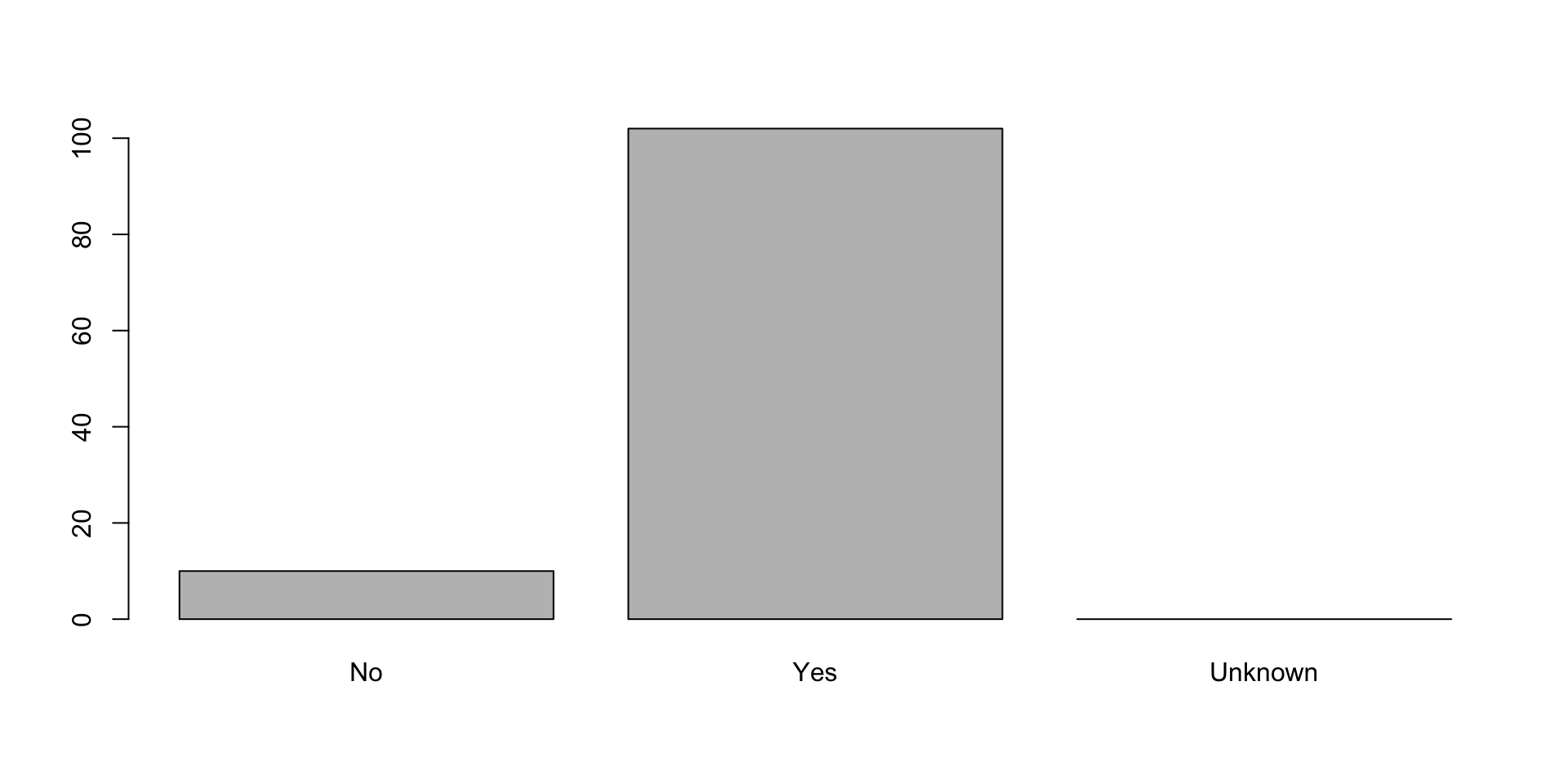
1. In the central_heating variable, rename “no”, “yes”, and “unknown” to “No”, “Yes” and “Unknown” respectively.
2. Recreate the barplot such that “Unknown” is last.

Solution

census_data$central_heating <- fct_recode(census_data$central_heating,
                              No = "no",
                              Unknown = "unknown",
                              Yes = "yes")

census_data$central_heating <- factor(census_data$central_heating, levels = c("No", "Yes", "Unknown"))

plot(census_data$central_heating)

Data wrangling with dplyr and tidyr

Learning objectives

• Subset columns or rows with select or filter and create new columns with mutate.
• Link the output of one function to the input of another function with the ‘pipe’ operator %>%.
• Use summarise, group_by, and count to split a data frame into groups of observations, apply summary statistics for each group, and then combine the results.
• Export a dataframe to a .csv and .tsv file.

Exercise 3.1

⏰ 5 mins

05:00

Using pipes, subset census_data to include responses from participants based in London and retain only the columns household_size, dwelling_type, and cars

Exercise 3.1 solution

census_data %>%
  filter(region == "London") %>%
  select(household_size, dwelling_type, cars)

Note that if you select before you filter, your code won’t run. That’s because you’re not retaining the variable that you use in your filtering. When piping, order matters!

Exercise 3.2

⏰ 10 mins

10:00

1. How many respondents lived in each dwelling_type?
2. Use group_by() and summarise() to find the median, min, and max number of bedrooms for each dwelling_type. Also add the number of observations (hint: see ?n)
3. What was the dwelling type with the most cars for each region?

Exercise 3.2 solution

1.
census_data %>%
    count(dwelling_type)

2. 
census_data %>%
    group_by(dwelling_type) %>%
    summarise(
        median_bedrooms = median(bedrooms),
        min_bedrooms = min(bedrooms),
        max_bedrooms = max(bedrooms),
        n = n()
    )

3.
census_data %>%
  drop_na(cars) %>%
  group_by(region) %>%
  filter(cars == max(cars))

Summary

• ✅ Subset columns or rows with select or filter and create new columns with mutate.
• ✅ Link the output of one function to the input of another function with the ‘pipe’ operator %>%.
• ✅ Use summarise, group_by, and count to split a data frame into groups of observations, apply summary statistics for each group, and then combine the results.
• ✅ Export a dataframe to a .csv and .tsv file.